CALCULATIONS AND FORTRAN CODE

All programs written by David Bisset, emphasizing utility rather than efficiency or elegance.

Determining the mounting axis direction for a reflector

The method is explained (with diagrams) in Section 3.1 of Ref [1]. For a given reflector, the program mirror-axis.for finds the values of the Cartesian components of its mounting axis direction vector, and the fixed angle between that axis and the reflector. The direction vector is a unit vector (only two independent components), so there are three unknowns including the fixed angle. The three numerically independent linear equations needed for solution are obtained from the dot product of the axis direction vector with the reflector mirror-normal vector. The latter changes with sun elevation, for which three values are selected as input.

Coordinate Axes: It is convenient for physical measurements if the X,Y axes lie in the planar face (if used) or in a tangent plane at the middle of a curved (e.g. paraboloidal) front face. The X-axis points towards (or directly below) the azimuthal position of the sun, the Y-axis is horizontal, and the Z-axis is orthogonally upwards. For the calculations, the origin is translated to the given reflector. The program assumes that the X,Y plane is horizontal, but adding an amount to each of the three sun elevations is equivalent to tilting the whole collector towards the sun by that amount. Example: Inputs for the uppermost reflector of the "Physical model with planar face" were 1222, -2150, 2703 for the position of the target as seen from that reflector, and 60, 90 and 120 for sun elevations (i.e. 15, 45 and 75 degrees sun elevations with collector face tilted 45 degrees).

Intersecting reflected rays with the target (receiver entrance)

These programs use REAL variables for controlling certain loops; my compiler lets me off with a warning. Rays are reflected from the centre of each reflector and all corners/vertices.

The programs model the physical rotation of a reflector about its axis after transforming vectors into a new set of coordinate axes. The new Y-axis is aligned in the negative direction of the reflector mounting axis, and the new X-axis lies in the original X-Y plane (horizontal). Transformations between coordinate axes follow Section 8.9 of Erwin Kreyszig, Advanced Engineering Mathematics (4ed, Wiley 1979).

The input file contains position, axis and angle data for the required reflectors in the form generated from MIRROR-AXIS runs. The final value in each line (defining the reflector-to-axis angle) is the "Constant" value from each run. Here's an extract from an input file (data for for three reflectors):
815 -1505 2760 -0.058604 0.978217 -0.199139 2.299664
815 -2350 2640 -0.069321 0.971746 -0.225618 1.796097
1222 -2150 2703 -0.097745 0.970121 -0.222062 1.887280
Output, for use in plotting software, is a file containing a list of intersection points (-y,-x) -- the axes are reversed so that the plot corresponds to a view of the target from below.

(a) Ideally curved reflector

For rectangular reflectors: image02.for
For hexagonal reflectors: image02hex.for

(b) Spherically curved reflector

For hexagonal reflectors: image02sphere.for

Sample calculations for finding absorber tube parameters

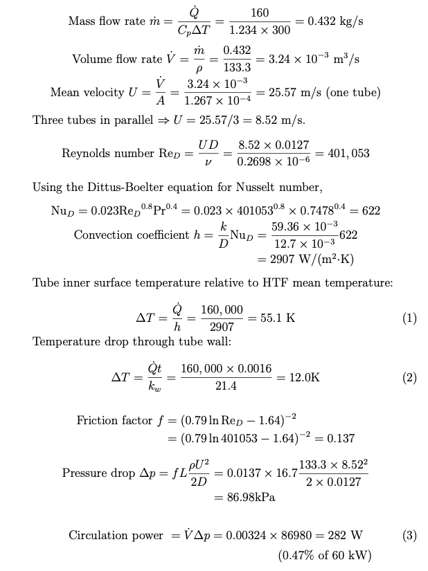
The following table, from Ref [1], demonstrates the feasibility of using a compressed gas as heat transfer fluid (HTF) in a bank of metal tubes within the cavity receiver. Critical aspects are the temperatures of the tubes and the pumping power required -- these aspects are inversely related. Calculations use the methods of Incropera and DeWitt, Fundamentals of Heat and Mass Transfer (4ed, Wiley 1996), Ch 8. Conditions of the fourth column of the table (CR = 200 and pressure = 200 bar) are used in the example calculations below; the number of tubes in parallel (and consequently their length) was selected after a few trials.

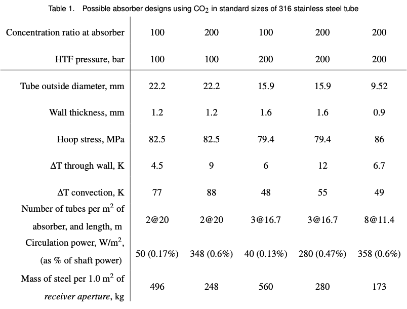
Some assumptions and data:

• Allowable hoop stress: The rupture stress at 649 C and 100,000 hrs for 316/316L stainless steel is 94 MPa (Product Data Bulletin at www.aksteel.com). Conductivity k = 21.4 W/(m.K) at 500 C.
• Data for CO2 at 500 C, 200 bar: density rho = 133.3 kg/m3; specific heat Cp = 1.234 kJ/(kg.K); conductivity k = 59.36E-3 W/(m.K); kinematic viscosity nu = 0.2698E-6 m2/s; Pr = 0.7478
• The 15.9 mm OD tubes are mounted in parallel at 20 mm centres. Internal X-sect area = pi x ((15.9/2)-1.6)^2 = 1.267E-4 m2
• Flux intensity of concentrated sunlight at the absorber is 160 kW/m2.
• Although the tubes could actually be staggered in more than one row, and their surfaces will receive variable heat flux by reflection and re-radiation as well as being at a range of angles to the incoming flux, the incoming flux intensity is used for calculations, applied to 20 mm of the tube circumference.
• The circulation power percentage assumes that 60 kW output is generated from 160 kW thermal input.
• Indicative temperatures: steam turbine inlet 540 C; molten salt hot tank 560 C; CO2 at inlet/exit 280/580 C; tube surface at exit 650 C.
• Calculations assume 1.0 m2 of absorber area.

The above results are a first approximation. They assume that less than half of the tube inner circumference participates in heat transfer, and that the tube is smooth and straight. Heat transfer enhancement could be applied inside the tubes in practice, and each tube will be divided into shorter lengths connected by U-joints or equivalent, which enhance heat transfer downstream. For example, if the collector front face is 50 x 100 m (area 5000 m2), the absorber area will be about 3.5 x 7 m (area 5000/200 = 25 m2); each 16.7 m length of tube could be divided into 5 subsections of nearly 3.5 m in an up-down-up-down-up flow configuration.

Updated April 2025.

*****************